Computer Methods in Applied Mechanics and Engineering · Volume 455 · Article 118912 · 2026

FNODE: Flow-matching for data-driven simulation of constrained multibody systems

Hongyu Wanga · Jingquan Wangb · Dan Negrutb,∗

a Department of Electrical and Computer Engineering, University of Wisconsin–Madison

b Department of Mechanical Engineering, University of Wisconsin–Madison

Received 18 Nov 2025 · Accepted 6 Mar 2026 · Available online 18 Mar 2026
doi:10.1016/j.cma.2026.118912 · ISSN 0045-7825 · ∗ Corresponding author

Paper arXiv preprint Code BibTeX
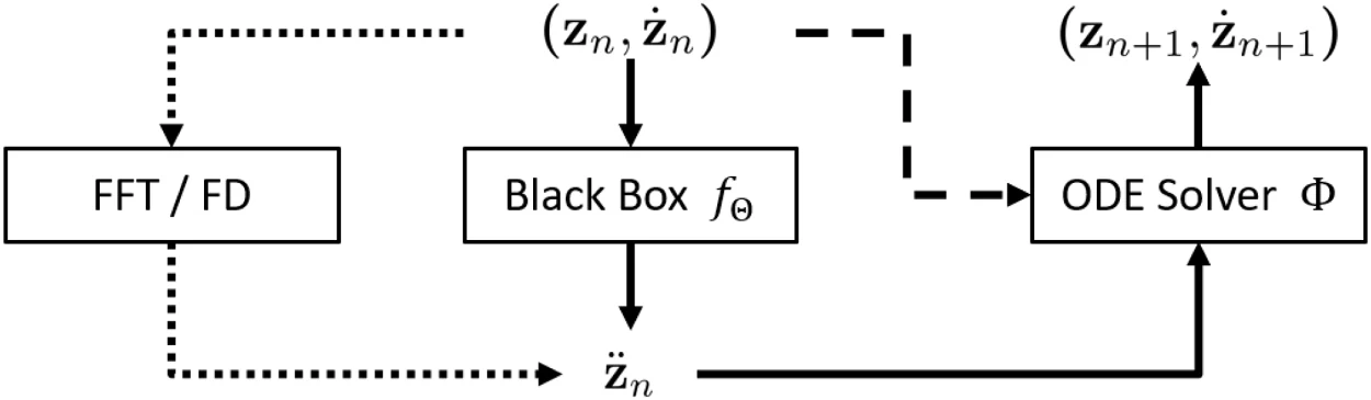
Block diagram of the FNODE forward pass: the state (z, ż) feeds an FFT/finite-difference block that produces target accelerations for training, and a neural network f_Θ whose predicted accelerations drive an ODE solver Φ that outputs the next state.
Fig. 1. Discretized forward pass of the FNODE framework for a general multibody dynamics (MBD) system. The solid arrows represent the data flow during both training and inference. The dashed arrows indicate latent inference operations. The dotted arrows denote the calculation of time derivative (training target). During training, “ground-truth” accelerations are computed from trajectory data using FFT- or finite-difference (FD)-based differentiation. Once trained, the neural model fΘ(⋅) predicts accelerations that are supplied to an ODE solver during inference to generate the system’s time evolution.
7.6×10⁻⁵
Rollout MSE on the single mass–spring–damper — 18× below MBD-NODE, three orders of magnitude below FCNN
≈ 2×
Lower wall-clock training time than MBD-NODE on every shared benchmark (Table 12)
0.46%
Energy drift over 30 s when the trained field is paired with a symplectic leapfrog integrator
18 → 2
Slider-crank states reduced to two learned coordinates by partitioning — constraints satisfied by construction

1. Overview

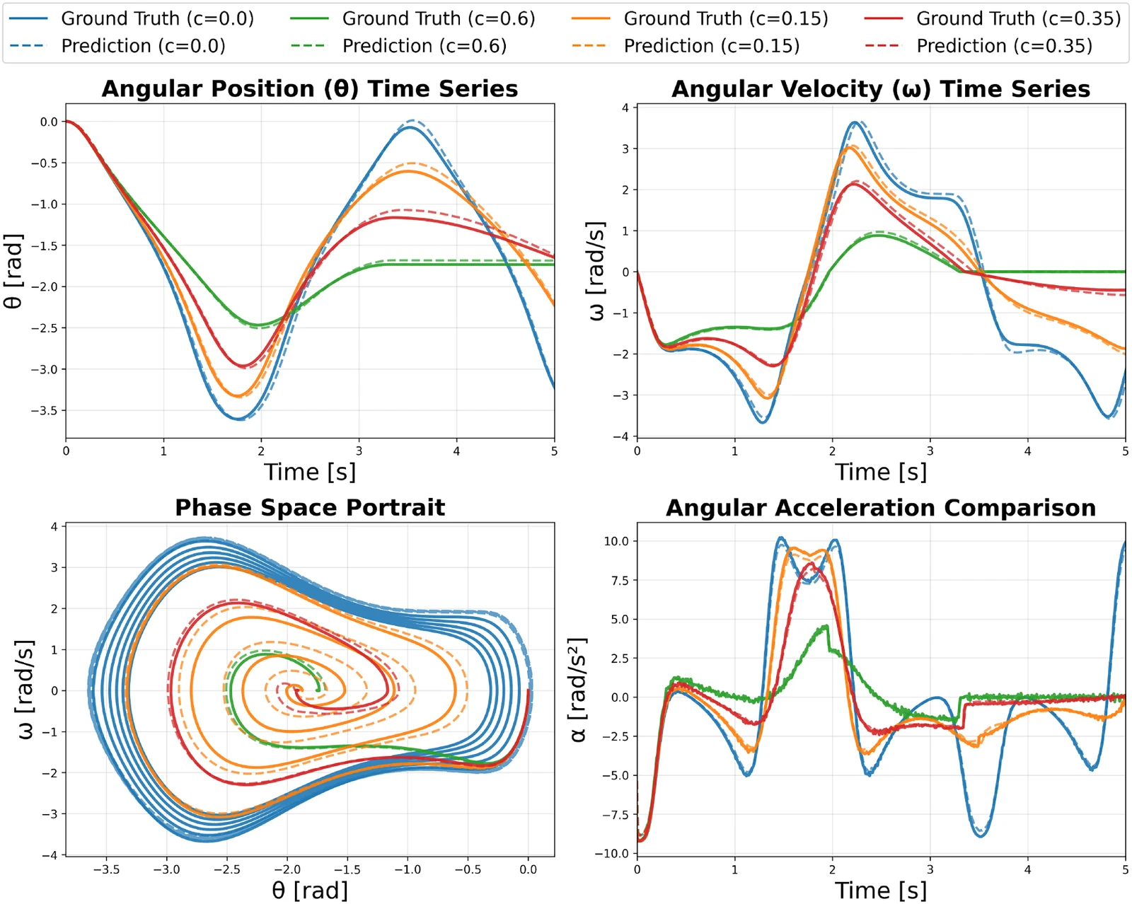
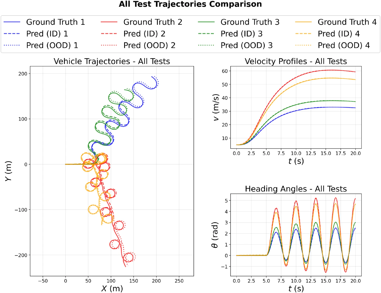
Data-driven modeling of constrained multibody dynamics faces two persistent obstacles: (i) the training cost of Neural ODEs, which typically backpropagate through an ODE solver, and (ii) error accumulation over long rollout predictions. We introduce FNODE, a Flow-Matching Neural ODE framework that learns the acceleration mapping directly from trajectory data. Because supervision targets accelerations rather than integrated states, training reduces to plain supervised regression — the ODE-adjoint/solver backpropagation bottleneck disappears. Acceleration targets are obtained efficiently by numerical differentiation, using a hybrid fast Fourier transform (FFT) and finite-difference (FD) scheme. Kinematic constraints are enforced through coordinate partitioning: FNODE learns accelerations only for the independent generalized coordinates, and the dependent coordinates are recovered by solving the position-level constraint equations. We evaluate FNODE on single and triple mass–spring–damper systems, a double pendulum, a slider–crank with and without friction, a vehicle model, and a cart–pole, comparing against MBD-NODE, LSTM, and fully connected baselines. On the single mass–spring–damper we also decompose the rollout error into the contributions of numerical differentiation and of the learned vector field: the network’s approximation error dominates, confirming that numerical differentiation of the training targets is robust. Across all benchmarks, FNODE improves both prediction accuracy and training and runtime efficiency, while the partitioning procedure maintains constraint satisfaction. Our code and scripts are released as open source to support reproducibility and follow-on research.

Keywords Multibody dynamics · Neural ODE · Constrained dynamics · Friction dynamics · Scientific machine learning · Flow-Matching

2. Method

2.1 Supervise accelerations, not states

A conventional Neural ODE obtains future states by solving an initial value problem, so every training step must differentiate through — or adjoint-solve alongside — the integrator. FNODE instead models the acceleration directly on the augmented state Z = (z, ): (t, μ) = fΘ(Z(t), μ), with μ an optional parameter input (e.g., a friction coefficient). Training is plain regression on the vector field,

ℒ(Θ) = (1/N) ∑if(zi, i; Θ) − i22,

with no ODE solve anywhere in the loop. The solver enters only at inference — and can be swapped freely: adaptive steppers for stiff phases, or symplectic leapfrog when energy behavior matters.
2.2 Hybrid FFT–FD acceleration targets

For smooth, near-periodic signals, spectral differentiation is highly accurate. A finite sampling window, however, breaks periodicity, and the resulting Gibbs error scales as ∼|Δboundary|/(2Δt) — independent of sample count, and growing as the step shrinks. The FFT pipeline therefore detrends, mirror-reflects with a cosine taper, applies a Tukey window (α = 0.2), and low-pass filters in the frequency domain (σ ≈ N/20).

Non-periodic data use finite differences: three-point central stencils in the interior (Ot2)) and one-sided stencils at endpoints (Ot)) — deliberately conservative, since wider stencils amplify noise. A Huber loss can absorb occasional label spikes without changing the architecture.

2.3 Constraints by coordinate partitioning

Constrained mechanisms evolve on the manifold of their kinematic constraint equations; learning accelerations for all redundant coordinates would let rollouts drift off it. Following the generalized coordinate partitioning of Wehage and Haug, FNODE learns the acceleration field only for the independent generalized coordinates; the dependent coordinates are recovered at every step by solving the position-level constraint equations — constraint satisfaction by construction.

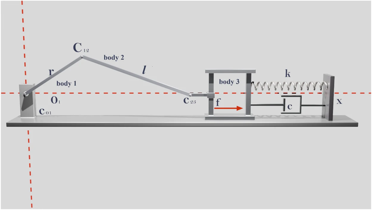
Concretely, the slider-crank’s 18-dimensional redundant state collapses to the two learned quantities (θ1, θ̇1); the kinematics return everything else.

2.4 An error budget that behaves

Rollout error separates into integrator truncation, learned-field mismatch, and differentiation-induced label error. An empirical decomposition on the single mass–spring–damper (15 step sizes, Δt ∈ [5×10⁻⁴, 10−2]) shows that the learned-field mismatch dominates — numerical differentiation of the training labels is not the bottleneck, whether the model is trained on analytical or finite-difference targets.

Every stage converges at its theoretical order: measured log–log slopes ≈ 3 for boundary FD, ≈ 4 for interior FD, and ≈ 8 for the RK4 trajectory MSE (Ot2p), p = 4).

3. Benchmarks and results

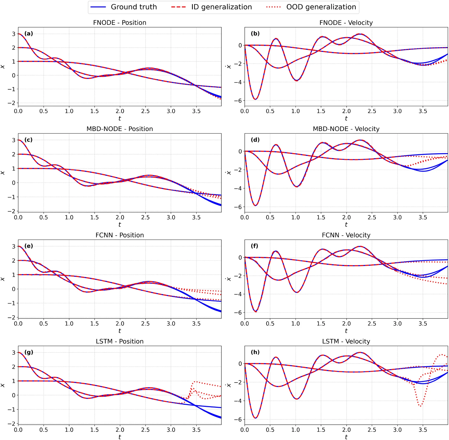
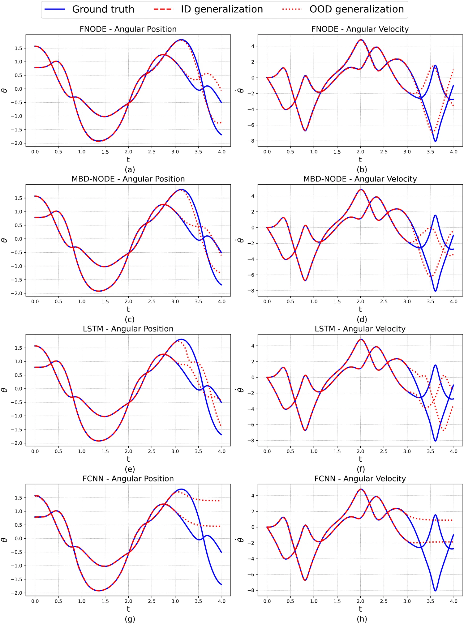
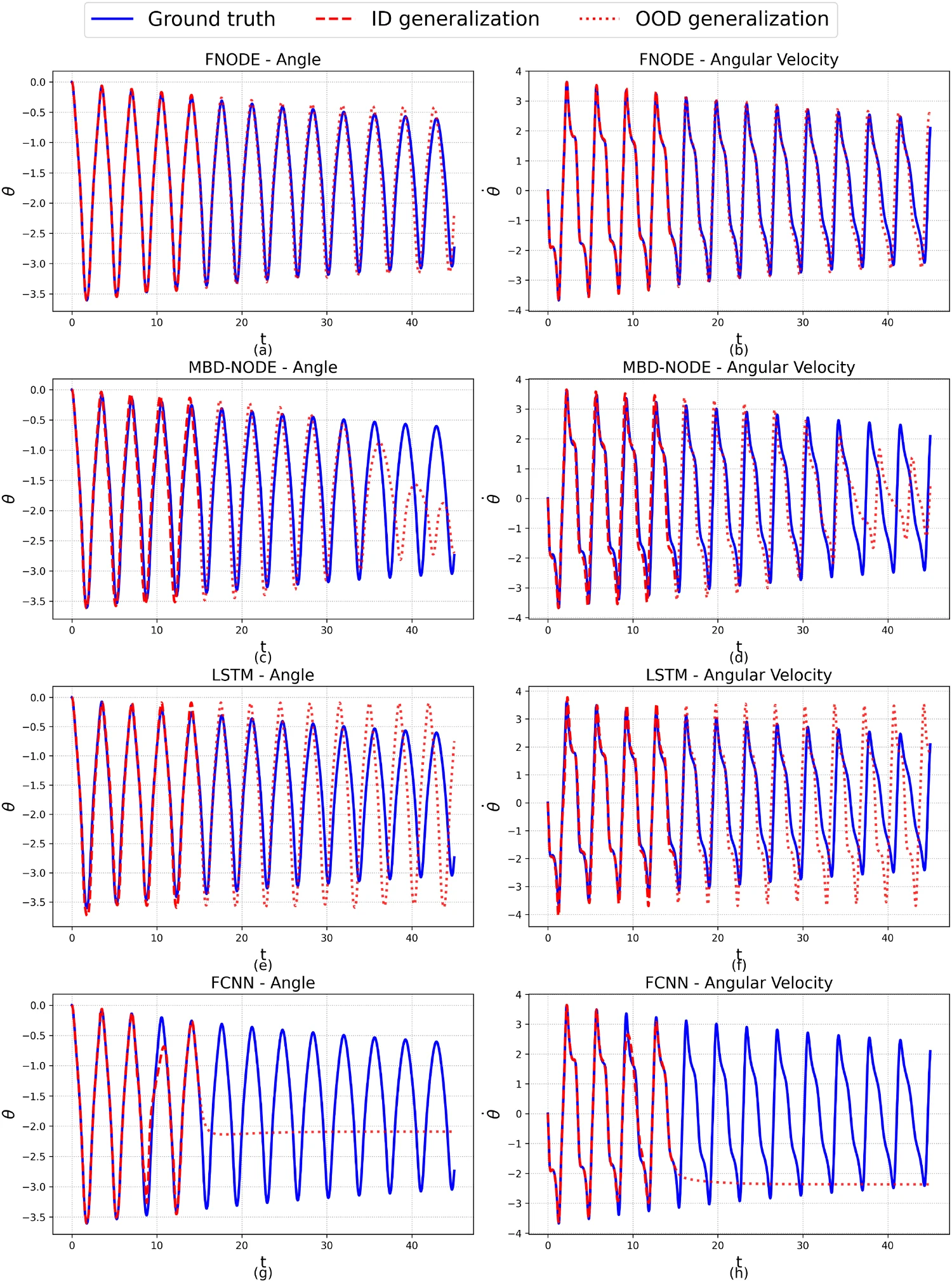
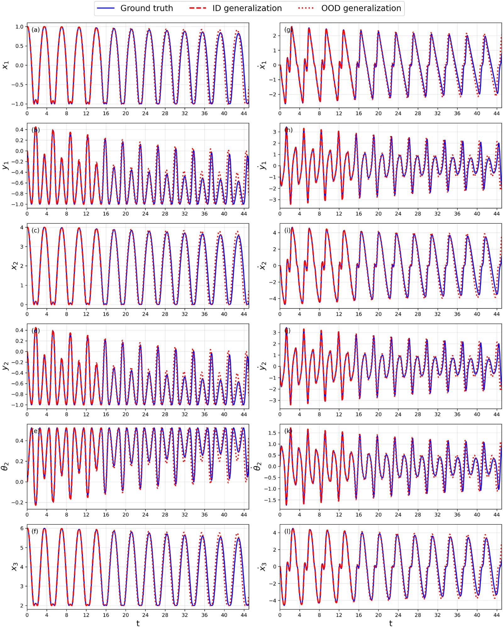
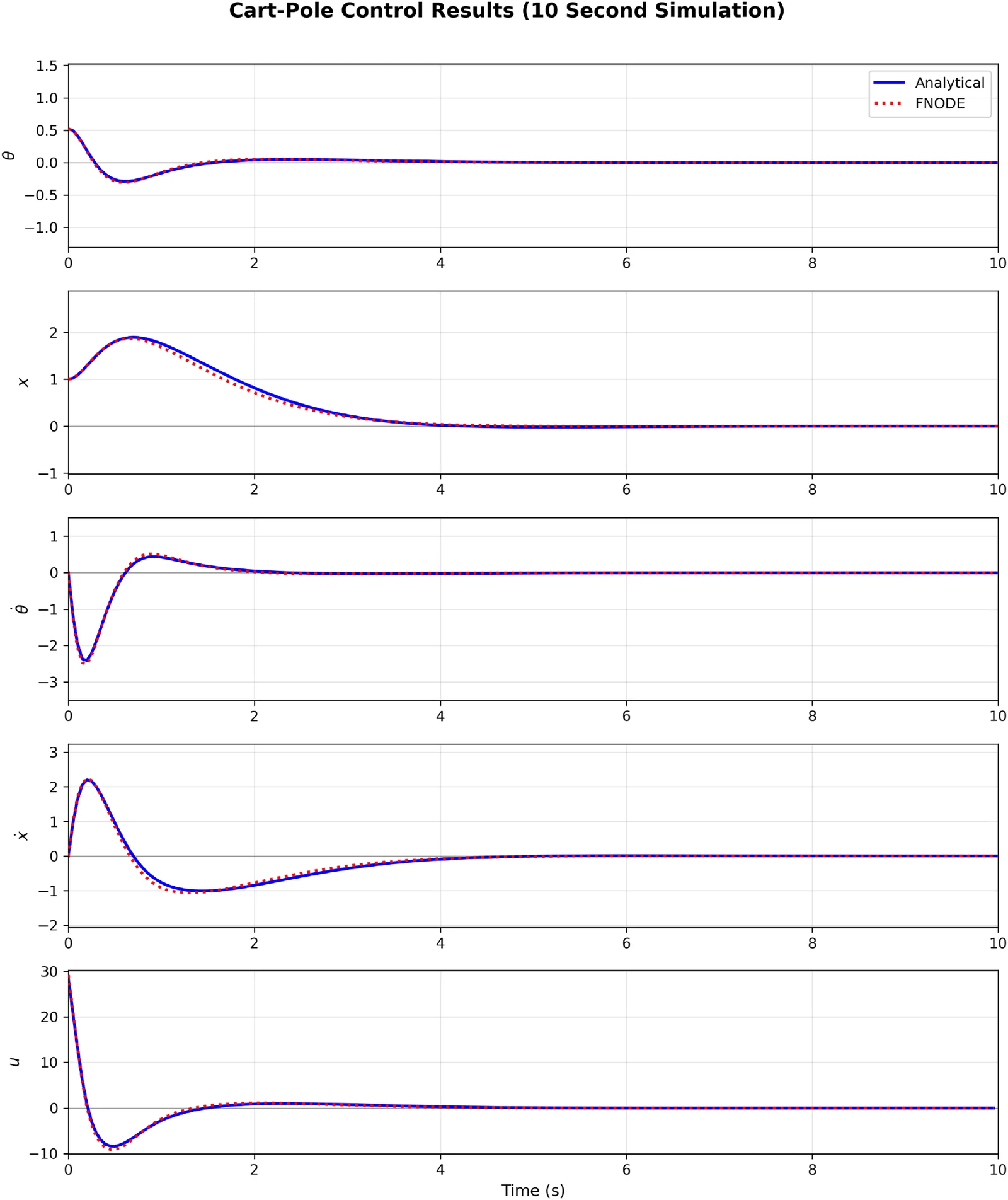
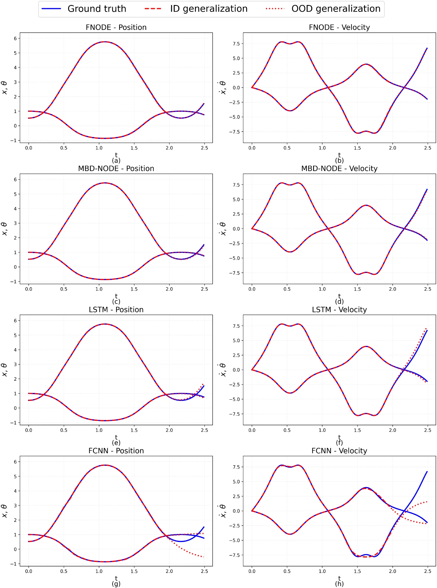
FNODE is evaluated on six mechanical systems of increasing difficulty against MBD-NODE, LSTM, and FCNN baselines — and, on the conservative oscillator, against Hamiltonian and Lagrangian Neural Networks as well. Figure and table numbers follow the published article; click any figure to enlarge it.

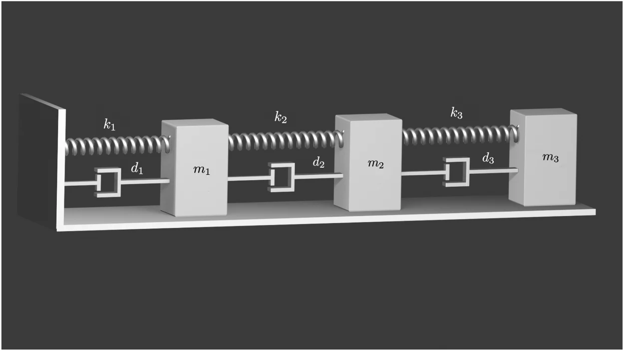
Rendered schematic of three masses connected in series to a wall by springs and dampers.
Fig. 7. Triple mass-spring-damper system. The setup is similar to the single mass-spring-damper system, except for the addition of two more masses, springs, and dampers. The system admits an analytical solution that was used for accuracy studies.
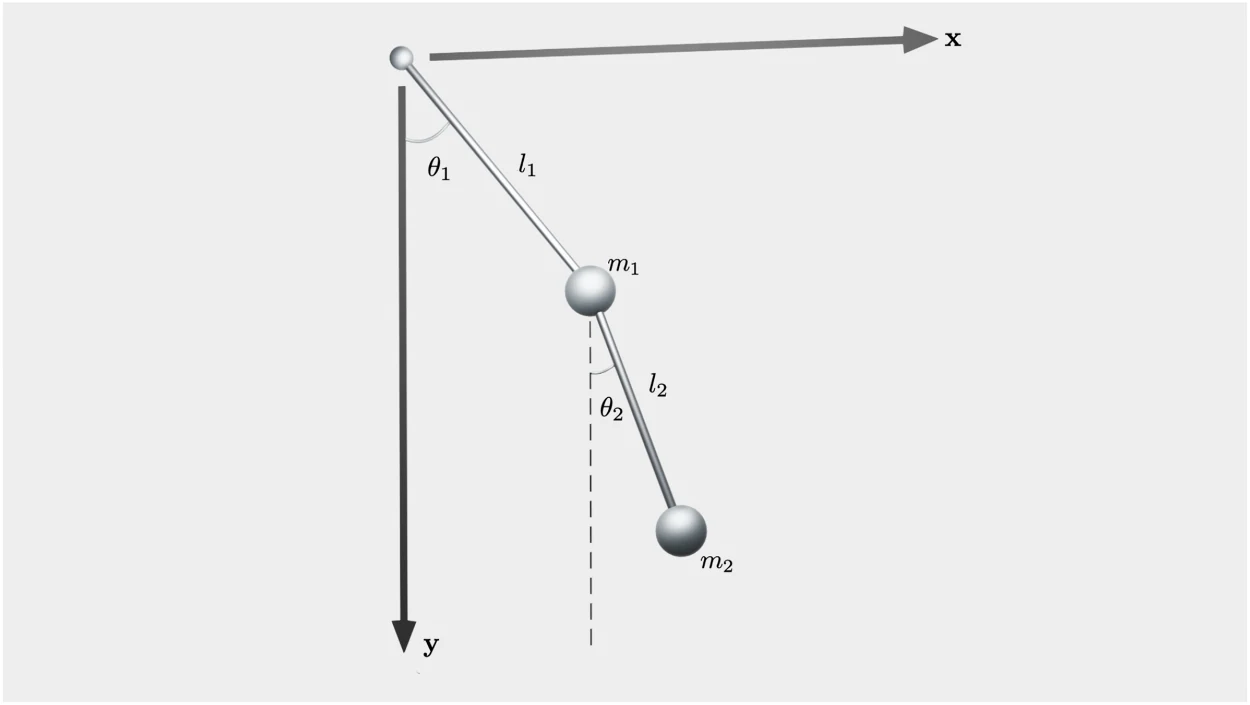
Schematic of a double pendulum with link lengths l1, l2 and angles θ1, θ2 measured from the vertical.
Fig. 10. Schematic of the double pendulum.
Rendered schematic of a slider-crank mechanism: crank, connecting rod, and slider with spring, damper, and friction force.
Fig. 13. Slider-crank mechanism with motor torque τ1, rotational dampers at all joints, and slider friction. The friction force is shown in red, see Appendix C, Eq. (C.5c), for its expression. It acts between body 3 and ground. (For interpretation of the references to colour in this figure legend, the reader is referred to the web version of this article.)
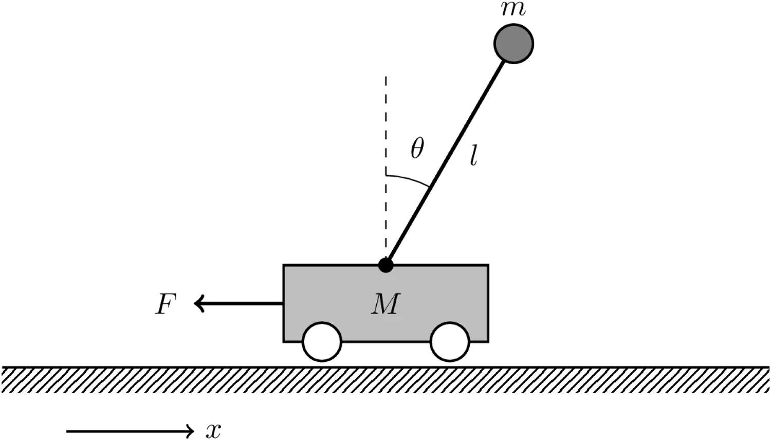
Line-drawing schematic of a cart-pole: cart of mass M under force F carrying a pole of length l at angle θ.
Fig. 21. Cart-pole system.
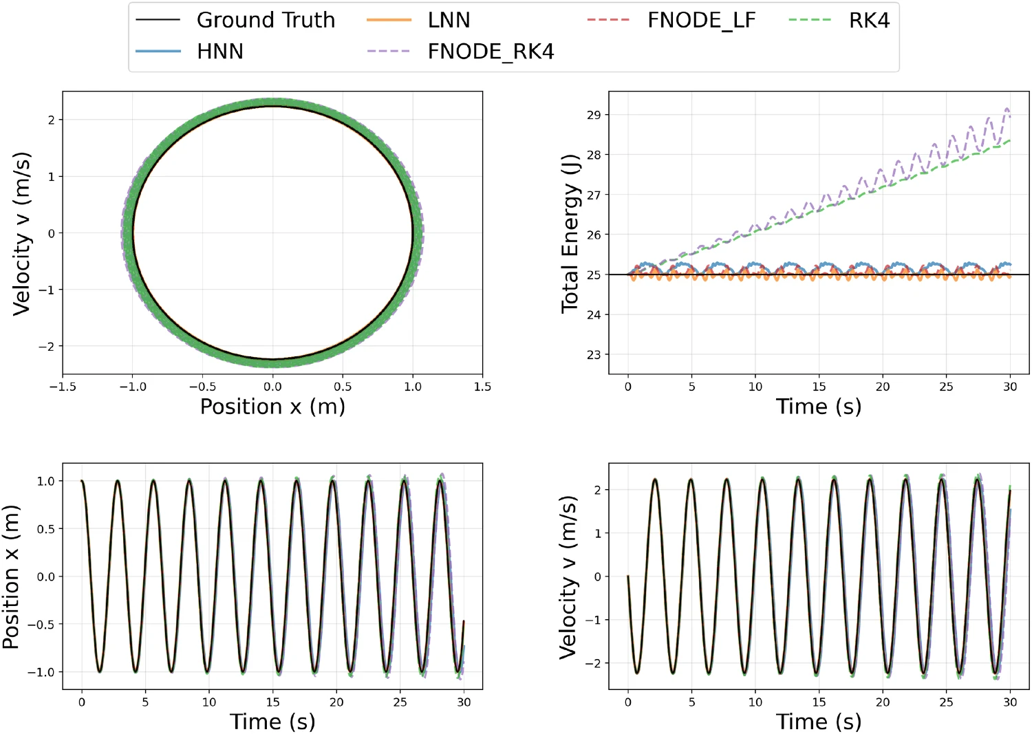
Four panels comparing ground truth, HNN, LNN, FNODE with RK4, FNODE with leapfrog, and RK4: phase portrait, total energy versus time, and position and velocity time series over 30 seconds.
Fig. 2. Phase-space trajectories and energy evolution for the single mass–spring system. The left panel shows the phase portrait (v vs. x), while the right panel shows the total energy. The energy drift ratios are: FNODERK4 (15.70%), FNODELF (0.46%), RK4 (13.39%), HNN (0.98%), and LNN (−0.24%). The mse for each model is provided: FNODERK4 (ε = 7.50e-2), FNODELF (ε = 9.66e-5), RK4 (ε = 2.02e-3), HNN (ε = 5.51e-2), and LNN (ε = 2.27e-4). The ground truth is provided by the analytical solution of the system.

Energy behavior over long horizons

The model is trained on 3 s of the undamped oscillator and rolled out for 30 s. Because the learned field is independent of the solver, it can be paired with any integrator after training: under a symplectic leapfrog scheme (FNODELF) it holds the energy drift to 0.46% and reaches the lowest MSE of all compared methods. It matches the structure-preserving HNN and LNN — in 450 training epochs where HNN needs 30,000. The same field under RK4 drifts like the classical RK4 baseline: the drift is an integrator property, not a modeling failure.

ModelMSEEnergy drift
FNODELF9.66×10−50.46%
LNN2.27×10−4−0.24%
RK4 (exact EOM)2.02×10−313.39%
HNN5.51×10−20.98%
FNODERK47.50×10−215.70%

4. Accuracy and efficiency

Across the five shared benchmarks, FNODE posts the lowest rollout MSE in the paper’s summary table — on most systems by an order of magnitude or more against the discrete-time baselines. Its training cost, meanwhile, stays on par with a plain FCNN, because no ODE solver sits in the backpropagation loop.

Table 13. Summary of numerical MSE (lower is better).
Test caseFNODEMBD-NODELSTMFCNN
Single mass–spring–damper7.6×10−51.4×10−31.5×10−21.6×10⁻¹
Triple mass–spring–damper6.1×10−36.8×10−32.5×10−19.0×10⁻²
Double pendulum1.4×10−12.3×10−17.6×10−11.9
Slider-crank1.7×10−18.7×10−11.43.1
Cart-pole6.7×10−41.1×10−31.6×10−13.5×10⁻¹
Table 12 (condensed). Wall-clock training time in seconds, Nvidia GeForce 5070 Ti (16 GB). MBD-NODE embeds an RK4 solver in its training loop; the vehicle baselines were not trained (dataset size prohibitive).
Test caseFNODEMBD-NODELSTMFCNN
Single mass–spring–damper112.46201.90171.99103.28
Triple mass–spring–damper108.23244.80172.05102.78
Double pendulum89.33212.09148.4188.04
Slider-crank565.011185.64813.11453.50
Cart-pole59.46144.5196.0859.36
4-DOF vehicle3304.32

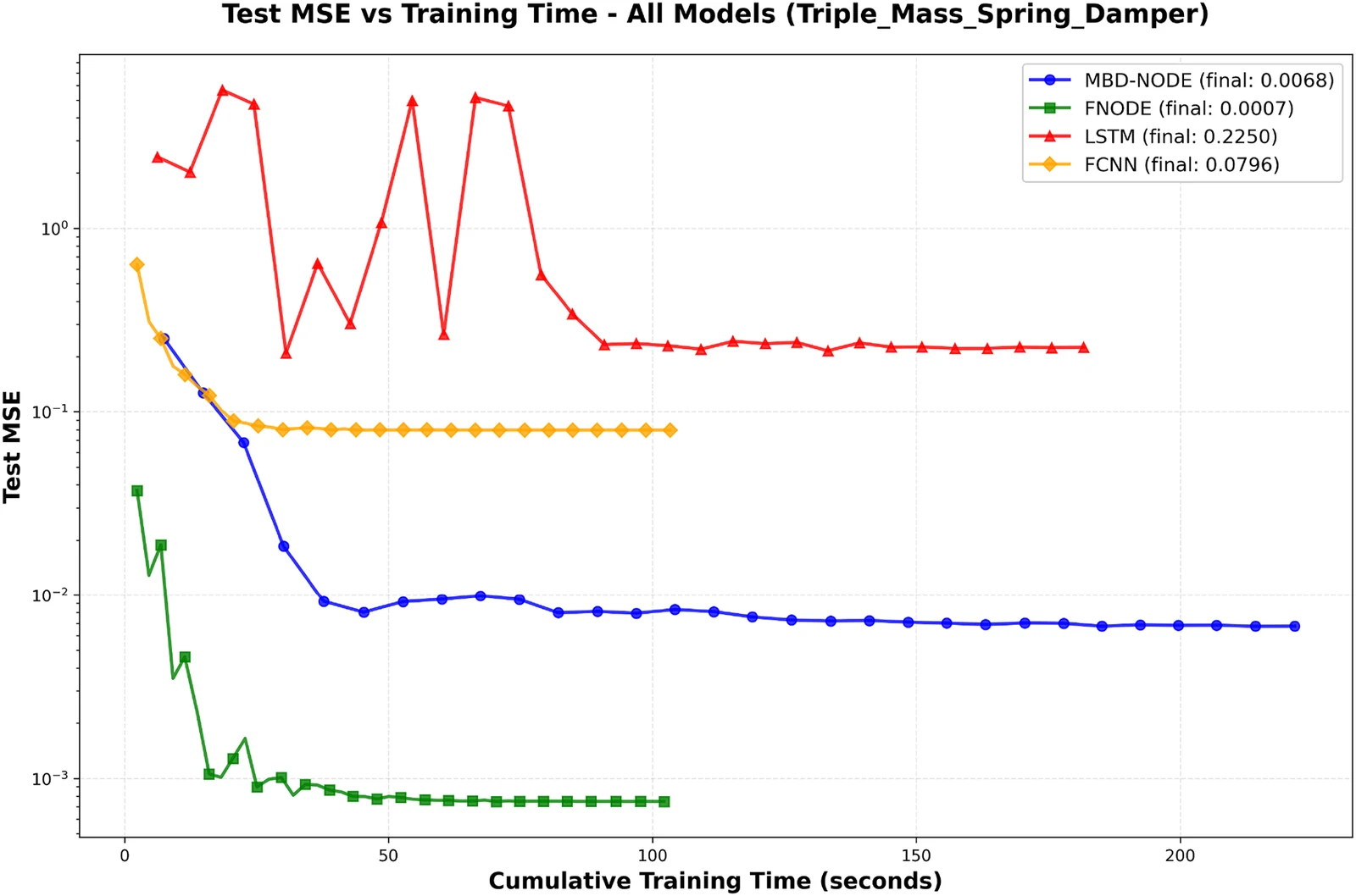
The accuracy–compute trade-off is summarized on the triple mass–spring–damper. In the test-loss-versus-training-time protocol of Fig. 26, FNODE’s error drops below 10−3 within roughly 50 s of cumulative training and settles at 7×10⁻⁴. MBD-NODE trains for over 220 s to reach its final 6.8×10⁻³, and the discrete-time baselines plateau roughly two orders of magnitude above FNODE’s settled error. (The rollout MSEs of Table 13 are computed under a separate evaluation protocol.)

Training setup common to the benchmarks

All models use 256 nodes per hidden layer, MSE loss, the Adam optimizer, and exponential learning-rate decay (0.98; 0.99 for FNODE on the slider crank); FNODE, MBD-NODE, and FCNN are fully connected with tanh activations, while the LSTM uses its sigmoid/tanh gating. Depth is tuned per system: two hidden layers for the mass–spring(–damper), double-pendulum, and cart-pole benchmarks, three for the slider crank, six for the 4-DOF vehicle (trained with AdamW at an initial learning rate of 10−4). FNODE and FCNN train for up to 450 epochs, MBD-NODE for 300–400, LSTM for 300; on the conservative single mass–spring benchmark, HNN requires 30,000 epochs. Complete per-system hyperparameter tables are given in the paper (Tables 2–6, 8, and 11).

Log-scale plot of test MSE versus cumulative training time for four models: FNODE converges fastest and to the lowest error; MBD-NODE, FCNN, and LSTM plateau at successively higher errors.
Fig. 26. The test MSE vs training time comparison of the all models on the triple mass-spring-damper benchmark.

5. Code and reproducibility

The complete implementation is released as open source in the Simulation-Based Engineering Lab reproducibility repository. It includes the FNODE training and evaluation pipelines; the MBD-NODE, FCNN, and LSTM baselines and the HNN/LNN references; ground-truth data generators and integrators for all six benchmark systems; and the friction-parameterized slider-crank, MPC cart-pole, and parameterized 4-DOF vehicle studies:

6. Citation

Hongyu Wang, Jingquan Wang, Dan Negrut, “FNODE: Flow-matching for data-driven simulation of constrained multibody systems,” Computer Methods in Applied Mechanics and Engineering, Volume 455, 2026, 118912, ISSN 0045-7825. doi:10.1016/j.cma.2026.118912

A preprint is available as arXiv:2509.00183. When using the code, please also cite the repository: H. Wang, J. Wang, D. Negrut, Models, scripts, and meta-data: FNODE, github.com/uwsbel/sbel-reproducibility, 2025.

@article{Wang2026FNODE,
  title   = {{FNODE}: Flow-matching for data-driven simulation
             of constrained multibody systems},
  author  = {Hongyu Wang and Jingquan Wang and Dan Negrut},
  journal = {Computer Methods in Applied Mechanics and Engineering},
  volume  = {455},
  pages   = {118912},
  year    = {2026},
  issn    = {0045-7825},
  doi     = {10.1016/j.cma.2026.118912}
}